Adaptive Recommender
A weekend playing with recommender systems: five different models, an engine that decides how much to listen to each one for each customer, and an evaluation that does not hide when the fancy idea only ties the simple one.
- why
- weekend project · to learn and have fun
- data
- 300 synthetic stores + Online Retail II (UCI, real data)
- task
- suggest products the store has not bought yet (next 92 days)
- models
- content · collaborative · supervised · Bayesian · popularity
- evaluation
- temporal validation · bootstrap CIs · paired comparisons
- interface
- 5-page Streamlit app · runs 100% locally
Which product should each store see?
Picture a clothing distributor that sells wholesale to stores: t-shirts, trousers, dresses, sportswear, accessories. Each store is a customer with its own taste — one sells sportswear, another only buys what is cheap, another concentrates its orders in summer. The distributor's sales rep wants to open the system and see, for each store, a short list of products it hasn't bought yet and probably would.
That is a recommender system: a program that ranks products from most to least likely to interest a customer and shows the top ones (here, the top 10). Two details change everything:
- Only products that are new to the store. Recommending what it already buys every week is easy and useless. The task is discovery.
- There is no single right way to guess. You can look at what the store bought, what similar stores buy, what is selling well, how it reacted to past suggestions… Each route works in different situations.
The question that got me started: what if, instead of picking one method, I used several and let the system decide how much to trust each one, customer by customer? That is called a mixture of experts. The rest of this page shows how I built it, one step at a time, and what happened when I tested it for real.
Nine stages, from raw data to a recommendation
Before the details, the map. The system is a sequence of stages; each one takes the previous one's output. Click each stage to see what it does and why:
Create the data. There was no real distributor data, so I wrote a synthetic data generator: 300 stores, 200 products, about 59 thousand order lines and 99 thousand interactions with recommendations over two years. The data is not random — each store has a "hidden taste" and its purchases follow it (details in section 03).
Then, to check I wasn't just rediscovering patterns I invented myself, I also ran everything on public real data (section 08).
Store it properly. Everything goes into a SQLite database with 19 tables: customers, products, orders, order lines, interactions, model versions, Bayesian estimates, displayed recommendations, weights used and evaluation results.
The database enforces integrity rules (no order for a non-existent customer, stock never negative, a weight must lie between 0 and 1), so a bug cannot silently corrupt the data.
Respect time. This is the most important care in the whole project. A model may only use what was known on the day the recommendation would be made. Train with October purchases to "predict" September and the result looks great and is a lie — that is called information leakage.
So all the code works with snapshots: "the data as it was on August 1st". If any later record shows up in a snapshot, the program stops with an error.
Turn history into numbers. Models don't read orders; they read numbers. For each store I compute characteristics such as number of orders, average order value, frequency, days since the last purchase and each category's share of purchases.
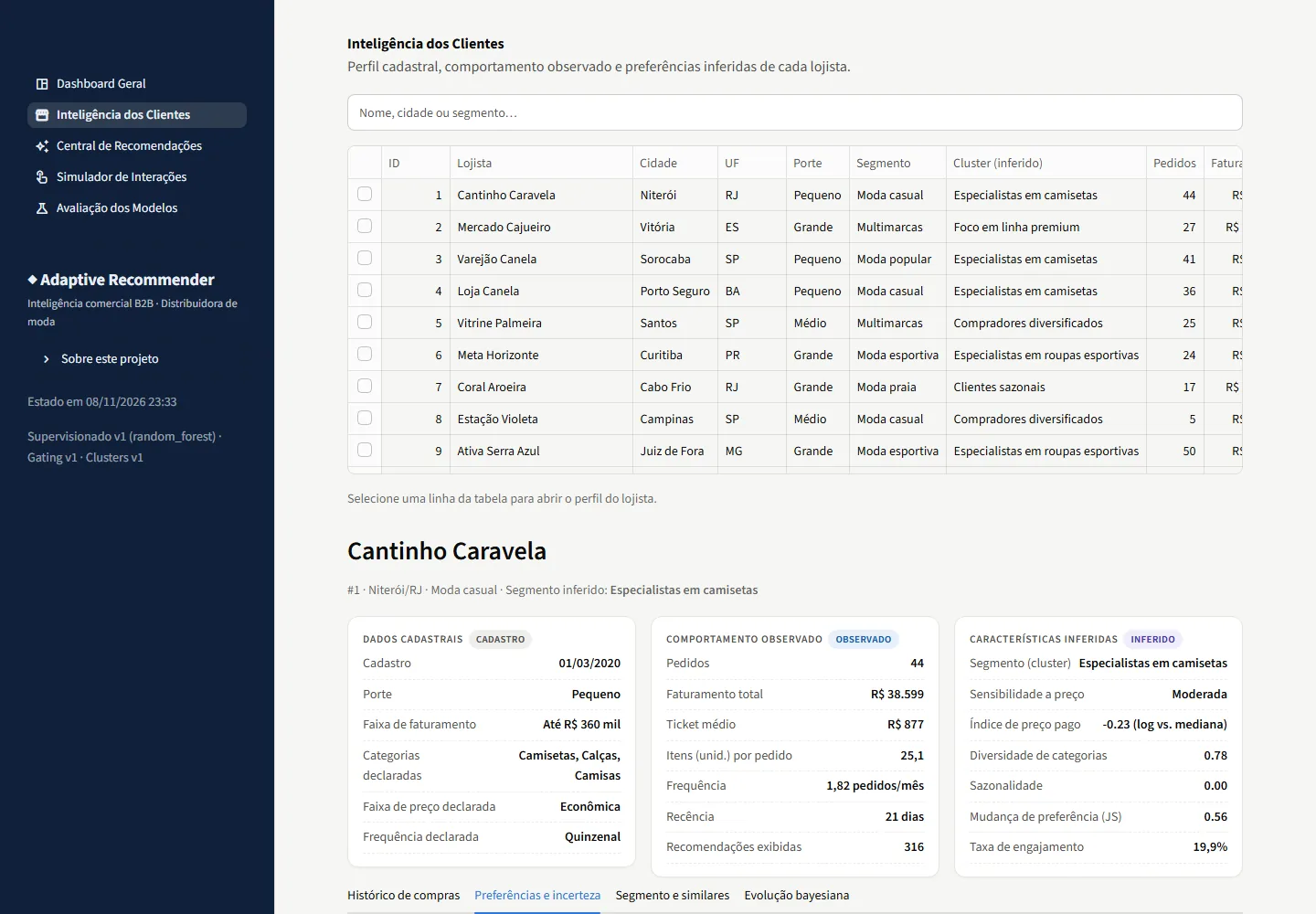
I keep two kinds apart: observed (counted directly, like "placed 44 orders") and inferred (depends on an assumption, like "is price-sensitive" or "changed taste recently"). In the app, each number carries a badge saying which kind it is.
Five ways to guess. Five different models each give a score to every store × product pair: content, collaborative, supervised, Bayesian and popularity (section 04 explains each one calmly).
They all share the same "plug": they take data up to a date, return a table of scores, say how confident they are for each store and can explain a score. That makes it possible to swap or add a model without touching the rest.
Decide how much to listen to each one. The five experts' scores live on different scales, so first they are put on a common 0–1 ruler. Then the adaptive engine picks weights that add up to 100% — different for each store — and takes a weighted average.
A brand-new store with no history gets a lot of weight on "popularity"; an old, consistent store gets more weight on "content" and "collaborative" (section 05).
Build the final list. Before ranking, I remove what cannot be suggested: products out of stock, not launched yet, already bought or recently rejected by the store. Then I rank, optionally diversify (so it doesn't suggest ten almost identical t-shirts) and write the reason for each suggestion.
Profit margin exists as a separate, optional objective: relevance to the customer and profitability for the company are never mixed unless you ask.
Learn from every reaction. When a store clicks, likes, adds to cart, buys or rejects a suggestion, the event is stored and the system immediately updates what it believes about that store — without retraining everything.
Each kind of reaction weighs differently: buying says much more than clicking, and just seeing a suggestion without reacting says almost nothing (section 06).
Test on the future. Models are trained on data up to April 2026, tuned on May–July and tested on August–October, a period none of them saw. We measure whether the suggested products were actually bought.
Every result comes with a confidence interval: with a few hundred stores, a small difference between two methods may just be luck (section 07).
A fake world with real rules
Made-up data is only useful for testing models if it has structure: patterns a good method can find and a bad method can't. So the generator doesn't draw purchases at random. It works like this:
1. Each store gets a hidden type (an archetype): sportswear specialist, price-sensitive, formal wear, seasonal (buys a lot in summer), diversified, high-ticket, "drifting" (slowly changes taste over time) and "complementary" (buys trousers together with shirts, dresses with accessories). The type sets its taste for categories and styles and how much price matters.
2. Each product has a "utility" for each store — a number saying how much it likes that product in that month. Simplified:
3. Orders happen over time. Every month each store places a random number of orders (a Poisson distribution, with more orders in "its" season) and picks products with higher probability for higher utility.
4. There is an old recommender showing 6 products before each order. The store reacts in a funnel: sometimes it clicks, sometimes adds to cart, sometimes buys, sometimes rejects — and most of the time it simply ignores. Those reactions become the interactions table.
5. New customers on purpose. Some stores only sign up at the end of the period — some never buy anything. That creates the cold-start problem: how do you recommend to someone with no history?
The crucial point: each store's hidden type lives in a separate file that no model reads. The models must discover the patterns from purchases, as they would in the real world.
Six ways of looking at the same customer
Each method answers a different question about the store. For each one: the intuition, how it works, the key formula and where it shines or fails. Click to switch:
the intuition
"When in doubt, suggest what is selling well." It is the simplest method and the baseline: any sophisticated method has to beat it.
how it works
For each product I count how many different stores bought it in the last 180 days, giving more weight to recent purchases (the weight halves every 60 days). The list is the same for every store.
where it shines and fails
Great for new stores we know nothing about. Weak for everyone else: it completely ignores each store's taste.
the intuition
"If the store buys gym leggings and sports tops, suggest other products similar to those." The method looks at product characteristics.
how it works
Step 1 — turn each product into a vector of numbers. Attributes like category, subcategory, audience, price band, material, colour and season become 0/1 columns (one-hot). The description text becomes numbers with TF-IDF, which gives high weight to rare, informative words ("gym", "corporate") and low weight to common ones.
Step 2 — measure similarity with the cosine, which looks at the angle between two vectors: 1 = pointing the same way (very similar), 0 = nothing in common.
Step 3 — build the store's profile: the sum of the vectors of the products it bought, weighting recent and larger purchases more. Likes and clicks add a little; rejections subtract. If the store changed taste recently, "forgetting" gets faster (a 60-day half-life instead of 180). A product's score is the cosine between it and the profile.
where it shines and fails
Works well with a consistent history and is the only method that can recommend brand-new products (nobody bought them yet). But it never surprises: it only suggests more of the same. A bonus: the explanation is exact — "42% of the score came from the category, 18% from the price band".
the intuition
"Stores that buy like you also bought this." It doesn't look at the product itself, only at who bought what.
how it works
Step 1 — the store × product matrix. A table with one row per store and one column per product; each cell says how much the store bought that product (recent purchases weigh more). Most cells are zero.
Step 2 — find the neighbours. Two stores are similar if their rows point the same way (cosine). Since stores with few products in common can look similar by chance, the similarity is "shrunk" when the overlap is small:
Step 3 — the neighbours vote. Take the 10 most similar stores; a product's score is the average of how much they bought it, weighted by similarity.
Variant tested: matrix factorization (ALS). Instead of neighbours, it summarizes each store and each product as 12 "hidden factors" whose product rebuilds the matrix. It shines on huge, sparse matrices; here it lost to the neighbours (0.207 vs 0.270), so it stayed as a comparison only.
where it shines and fails
It finds patterns no product attribute reveals. But it doesn't work for stores with no history (nobody to compare them to) or for products nobody has bought.
the intuition
Turn recommendation into a yes/no question: "will this store buy this product in the next 92 days?" — and train a machine learning model to answer with a probability.
how I built the examples
I go back in time month by month. At each date, for every store × product pair not yet bought, I compute 43 features (about the customer, the product and the pair, such as "the category's share of the store's purchases") using only data before that date. The label is 1 if the purchase happened in the next 92 days, 0 otherwise.
An important statistical care: "didn't buy" doesn't mean "doesn't like" — maybe the store never saw the product. So (a) the label only holds for that window, (b) only stores that placed some order in the window are included, i.e. that had a chance to buy, and (c) whether the store had already seen, clicked or rejected the product is itself a feature.
Since only ~4% of pairs are purchases, I sample the "no"s and give each one a weight equal to the inverse of the sampling rate — that keeps the probabilities correct.
the models
I train three — logistic regression (linear and interpretable), random forest (an average of many trees) and LightGBM (trees in sequence, each fixing the previous one's errors) — and keep the best on a validation period. Then I apply Platt calibration, which adjusts the probabilities so that "30%" really means about 30% purchases.
where it shines and fails
It is the best single expert (NDCG@10 0.289), because it combines all signals and learns from every store — it even makes reasonable guesses for new stores. The price: slower to train and less transparent than the others.
the intuition
Answer "when we suggest dresses to this store, does it usually respond well?" — and, above all, how sure are we. A store that responded well 2 times out of 2 is very different from one that did 200 times out of 200.
the Beta distribution
The response rate θ is unknown, so it is treated as a variable with a Beta(α, β) distribution. Think of α as "imaginary successes" and β as "imaginary failures"; the mean is α/(α+β) and the larger α+β, the narrower (more certain) the distribution.
The big advantage is the conjugate update: observed s successes and f failures? Just add them.
two stages and weighted evidence
I model the funnel in two steps, per store × category: interest (did it respond positively to the suggestion?) and conversion (given interest, did it buy?). The purchase probability is the product of the two. Each reaction counts differently:
- purchase: success in both stages — the strongest evidence;
- click or "like": success in interest, failure in conversion;
- explicit rejection: a full failure in interest;
- seen and ignored: only 0.25 of a failure in interest — maybe the store barely noticed it. Ignoring is not rejecting.
where the starting point (prior) comes from
Before any interaction, a store's estimate starts from the average of stores in the same segment (excluding itself), pulled towards the overall average when the segment has little data. How strong that starting point is gets estimated from the data itself (empirical Bayes).
where it shines and fails
It shows uncertainty honestly (credible intervals in the app) and learns instantly from every click. But it works per category, not per product: it says "dresses work for this store", not "which dress". On its own it is weak (0.185) — its job is to add a complementary signal.
the intuition
Group similar stores — "sportswear specialists", "price-sensitive", "seasonal" — not to recommend directly, but to give context to the other models (the Bayesian starting point and one of the supervised features come from here).
how it works
Each store becomes a point with average order value, frequency, category diversity, price sensitivity, recency, seasonality and each category's share — all standardized to the same scale. K-Means finds k centres and puts each store in the group of the nearest centre, minimizing:
how many groups?
I try k from 2 to 10 and pick by the product of two criteria: silhouette (are the groups well separated?) and stability (if I resample the stores and run again, do the groups hold?). I also compare with another algorithm, Ward's hierarchical clustering. Group names are generated automatically from what sets each centre apart from the average.
where it shines and fails
It gives vocabulary and context. Stores with fewer than 3 orders are not clustered — they get "not enough history" instead of an arbitrary label.
How the system decides how much to listen to each expert
This is the part I most wanted to test. Instead of the same fixed weights for everyone, each store gets its own weights. Five steps:
1. Put the scores on the same ruler. Content's score is a cosine, supervised's is a probability, popularity's is a count — mixing them directly would be adding metres to kilograms. So, for each store, I replace each score by its rank among the possible products, converted to 0–1 (a percentile). An expert that gives everything the same score becomes 0.5 everywhere and doesn't disturb the order.
2. Measure what we know about the store. Number of orders and of distinct products, how many suggestions it has seen, how similar it is to other stores, how consistent its history is, whether it changed taste recently, how many days since it last bought.
3. Common-sense rules. Each signal becomes a confidence between 0 and 1 for each expert: few orders → little trust in collaborative; consistent history → more content; many similar neighbours → more collaborative; many interactions → more Bayesian and supervised; new store → more popularity. Weights are the confidences divided by their sum.
4. A learned adjustment on top of the rules. The rules are my guesses. So a small model learns corrections to them by looking at what worked in a past period:
Here \(r_e\) is the rule's confidence, \(b_e\) a general adjustment per expert and \(\theta_e\) adjustments that depend on the store's signals \(\phi\). If learning finds nothing, \(b = \theta = 0\) and the system falls back exactly to the rules. The "softmax" guarantees positive weights that add up to 100%.
5. Don't trust the adjustment blindly. With few stores, a 60-parameter model can memorize noise. So I compare, with cross-validation (training on some stores and testing on the others), three versions — rules only, general adjustment only, full adjustment — and keep the one that does best outside the training data. With 50 stores the rules won; with 300 the full adjustment won.
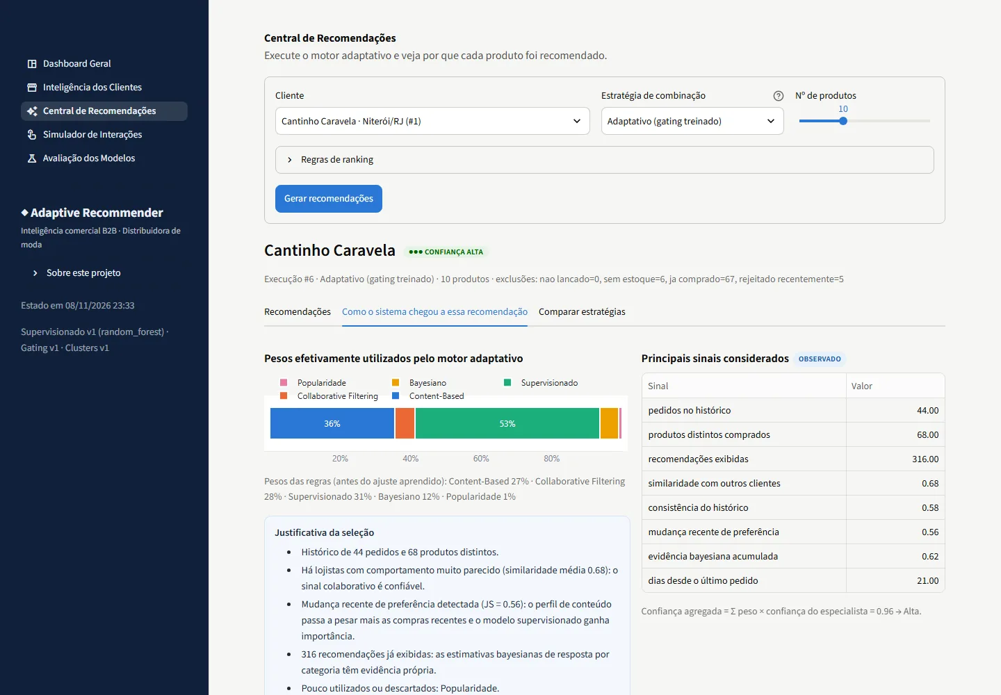
Every recommendation shows the weights used, the justification in plain language, the discarded experts and a confidence level (fig. 3).
From score to list — and what happens after a click
Filter before ranking. Left out: products out of stock, not launched yet, already bought by the store (there is an option to allow repurchase after N days) and rejected in the last 180 days. Products shown several times without any response lose 15% of their score ("fatigue"), so the list doesn't get repetitive.
Diversify, if you want. With Maximal Marginal Relevance, each next item balances relevance against being different from what is already on the list:
With λ = 1 the list is pure relevance; smaller values bring more variety.
Learning from a click — an example. Suppose a store's Bayesian interest estimate for "dresses" is Beta(3, 7): mean 3/10 = 30%. The store sees a dress suggestion and…
- …clicks: it becomes Beta(4, 7), mean 4/11 ≈ 36%;
- …ignores it: Beta(3, 7.25), mean ≈ 29% — almost nothing changes, because ignoring is weak evidence;
- …rejects it: Beta(3, 8), mean 3/11 ≈ 27%.
If after the click the same store buys the dress, the system applies only the difference between "clicked" and "bought", so the same suggestion isn't counted twice. Thanks to that, updating one event at a time gives exactly the same result as recomputing everything from scratch — that is checked in the tests.
What changes right away and what waits for retraining. After feedback, these update immediately: the Bayesian estimate, the store's features, its content profile, its row in the collaborative matrix and the engine's weights. The supervised model, the factorization, the segments and the trainable engine are only refitted in a controlled retraining routine, which creates new versions and never deletes data.
Did it work? Measuring without fooling yourself
The protocol. Train on data up to April 2026, use May–July to choose hyperparameters and train the engine, test on August–October. For the test, the models are refitted with everything up to July 31st, but the engine uses the weights learned before — nobody sees the test period.
The metrics, for each store's top-10 list:
- Precision@10: of the 10 suggested, how many the store actually bought.
- Recall@10: of the new products the store bought, how many were on the list.
- NDCG@10: like recall, but rewarding hits at the top — a hit in 1st place is worth more than in 10th. Ranges from 0 to 1.
- Coverage: what share of the catalogue appears in some list (always suggesting the same 20 products is a bad sign).
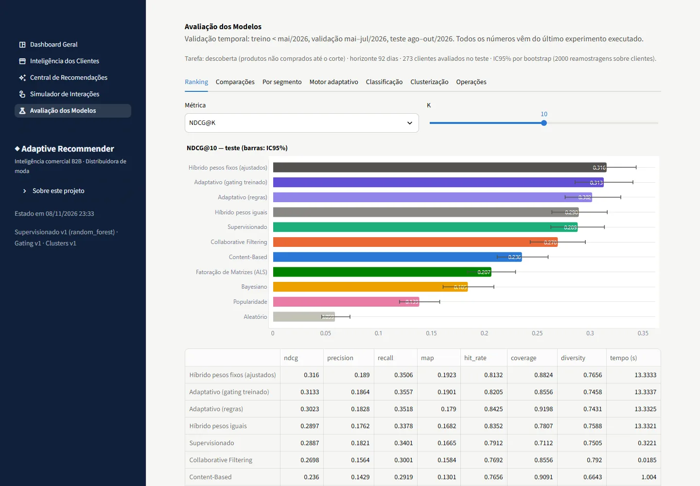
Uncertainty. With 273 stores in the test, part of the difference between two methods is luck. The bootstrap estimates it: draw 2,000 sets of 273 stores with replacement, recompute the average and see the range it moves in (the 95% interval). To compare two methods, do the same with the difference between them store by store (paired bootstrap): if the difference's interval includes zero, you can't say one is better.
| strategy | NDCG@10 | 95% CI | recall@10 | precision@10 | coverage |
|---|---|---|---|---|---|
| Hybrid · fixed weights | 0.316 | [0.287, 0.343] | 0.351 | 0.189 | 0.88 |
| Adaptive · trained gating | 0.313 | [0.286, 0.340] | 0.356 | 0.186 | 0.86 |
| Adaptive · rules | 0.302 | [0.276, 0.329] | 0.352 | 0.183 | 0.92 |
| Hybrid · equal weights | 0.290 | [0.264, 0.316] | 0.338 | 0.176 | 0.78 |
| Supervised | 0.289 | [0.263, 0.313] | 0.340 | 0.182 | 0.71 |
| Collaborative (kNN) | 0.270 | [0.243, 0.295] | 0.300 | 0.156 | 0.86 |
| Content | 0.236 | [0.212, 0.260] | 0.292 | 0.143 | 0.91 |
| Factorization (ALS) | 0.207 | [0.184, 0.229] | 0.262 | 0.136 | 0.93 |
| Bayesian | 0.185 | [0.161, 0.209] | 0.202 | 0.105 | 0.98 |
| Popularity | 0.139 | [0.120, 0.158] | 0.152 | 0.098 | 0.30 |
| Random | 0.059 | [0.046, 0.073] | 0.069 | 0.038 | 1.00 |
The comparisons that matter. The "reading" column applies the rule above, with no interpretation from me:
| comparison (A − B) | Δ NDCG@10 | 95% CI | reading |
|---|---|---|---|
| Adaptive · trained gating − Hybrid · fixed weights | −0.003 | [−0.019, +0.014] | tie — the interval includes zero |
| Adaptive · rules − Hybrid · fixed weights | −0.014 | [−0.029, +0.003] | tie — the interval includes zero |
| Adaptive · trained gating − Adaptive · rules | +0.011 | [−0.002, +0.023] | tie — the interval includes zero |
| Adaptive · trained gating − Supervised | +0.025 | [+0.006, +0.043] | A better — consistent difference |
| Adaptive · rules − Supervised | +0.014 | [−0.007, +0.035] | tie — the interval includes zero |
| Hybrid · fixed weights − Supervised | +0.027 | [+0.003, +0.050] | A better — consistent difference |
| Adaptive · trained gating − Hybrid · equal weights | +0.024 | [+0.011, +0.037] | A better — consistent difference |
| Supervised − Popularity | +0.150 | [+0.123, +0.177] | A better — consistent difference |
| Collaborative (kNN) − Factorization (ALS) | +0.063 | [+0.042, +0.085] | A better — consistent difference |
By amount of history. One of the adaptive engine's promises was to do better for new stores. The data says:
| stores | n | popularity | supervised | fixed weights | adaptive |
|---|---|---|---|---|---|
| long history | 204 | 0.117 | 0.284 | 0.314 | 0.317 |
| moderate history | 35 | 0.163 | 0.284 | 0.297 | 0.286 |
| short history | 16 | 0.233 | 0.370 | 0.416 | 0.406 |
| no history | 18 | 0.259 | 0.275 | 0.285 | 0.247 |
Test NDCG@10 by how much history the store had at recommendation time. Small groups (n < 20) are indicative, not conclusive. Source: docs/MODEL_EVALUATION.md.
What I conclude. Combining experts really helps: the hybrids beat every single expert with statistical room to spare. But the adaptive engine — the most sophisticated part — ties a simple blend of well-chosen fixed weights (Δ = −0.003, interval −0.019 to +0.014), and loses to it on stores with no history. That is why it is not claimed to be better.
The lesson I liked most. I started with 50 stores. There, the trainable engine couldn't learn anything (cross-validation always picked the rules) and a nice advantage for the adaptive engine showed up on "stores that changed taste" — with 7 stores in that group. Going up to 300 stores, the confidence intervals became more than twice as narrow, the engine started learning… and the advantage vanished. It was noise. Had I stopped at 50 stores, I would have had a pretty, false conclusion.
And outside the world I invented myself?
Synthetic data has a basic problem: I created the patterns. To check, I ran the same code, without changing any model, on Online Retail II (UCI Machine Learning Repository): real 2009–2011 transactions from a UK online wholesaler whose customers are largely resellers — a similar B2B setting.
- Cleaning: from 1,067,371 rows I removed cancellations, returns, anonymous customers and codes that aren't products (postage, adjustments, bank charges), keeping 802,632.
- Adaptation: the dataset has no categories, so they are derived from the descriptions with keywords (bags, kitchen, candles, Christmas…). I used the 400 products with the most buyers before the validation period and a random sample of 500 customers — 58 of them only appear in the test period (real cold start).
- What's missing: there are no recommendation logs, so the Bayesian expert has no evidence of its own.
| strategy | NDCG@10 | 95% CI | recall@10 | precision@10 | coverage |
|---|---|---|---|---|---|
| Hybrid · fixed weights | 0.094 | [0.076, 0.112] | 0.086 | 0.066 | 0.39 |
| Supervised | 0.091 | [0.072, 0.111] | 0.082 | 0.061 | 0.66 |
| Hybrid · equal weights | 0.085 | [0.068, 0.104] | 0.087 | 0.067 | 0.30 |
| Collaborative (kNN) | 0.085 | [0.069, 0.101] | 0.090 | 0.063 | 0.84 |
| Adaptive · trained gating | 0.084 | [0.066, 0.102] | 0.088 | 0.065 | 0.38 |
| Factorization (ALS) | 0.081 | [0.063, 0.100] | 0.080 | 0.059 | 0.95 |
| Adaptive · rules | 0.080 | [0.062, 0.099] | 0.079 | 0.061 | 0.67 |
| Bayesian | 0.073 | [0.058, 0.089] | 0.058 | 0.058 | 0.09 |
| Popularity | 0.070 | [0.055, 0.085] | 0.058 | 0.060 | 0.09 |
| Content | 0.069 | [0.053, 0.086] | 0.068 | 0.052 | 0.86 |
| Random | 0.034 | [0.025, 0.044] | 0.026 | 0.028 | 1.00 |
Reading. All numbers drop — real data is much sparser (the median customer has 3 orders) — but the story repeats: every method beats chance comfortably, and the best strategies (fixed weights 0.094, supervised 0.091, collaborative 0.085, adaptive 0.084) are statistically tied. Content suffers from short descriptions and the Bayesian expert, without interactions, becomes almost a popularity model. No magic — which, to me, is good news about the honesty of the evaluation.
Everything in an interface you can explore
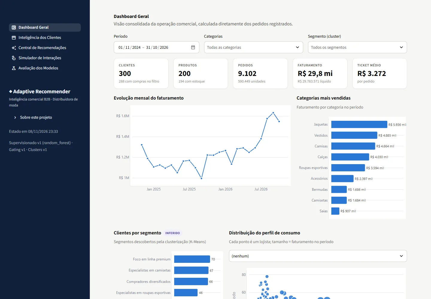
A five-page Streamlit app runs everything locally: sales dashboard, customer intelligence (with observed and inferred data marked differently), a recommendation center that explains the weights, an interaction simulator (every click is stored and really updates the models) and an evaluation lab with all the charts above.
Lessons and limits
- The evaluation setup matters more than the model. Splitting by time, comparing against fair baselines and showing uncertainty is what kept me from believing a false conclusion.
- Sample size decides what can be learned. The same trainable engine learned nothing with 50 stores and did with 300.
- Sophistication is no guarantee. An adaptive engine with rules, softmax and cross-validation tied five well-chosen fixed weights. In production, I would start with fixed weights.
- Ignoring is not rejecting. Treating a missing click as "dislikes it" would have distorted the Bayesian and supervised models.
- Limits: the main data is synthetic (the generator defines the "truth"); some models are over-engineered for ~300 customers — on purpose, it was a playground; small-group results (like cold start) are indicative; the Bayesian expert only works where interaction logs exist.
Personal weekend project, built to learn. Real data: Online Retail II (Chen, D., UCI Machine Learning Repository, CC BY 4.0), downloaded at runtime and not redistributed.